Jiro's pick this week is Simulink GUI Synchronization by our fellow MathWorker Will Campbell.

Here's a little something new. We've been mostly looking at MATLAB entries in this blog, but today we'll take a look at a Simulink example. Even though this is a simple example, I find this very useful and pedagogical. Imagine that you want to build a graphical user interface that controls your Simulink model (You know how I'm all about GUIs!). This is not uncommon and can be accomplished by using functions like set_param and get_param. But what if you want to be able to control the model directly through Simulink as well as through the MATLAB interface? In that case, you want to make sure that the interface accurately reflects the current state of the model.

In this example, Will shows how you can create a MATLAB GUI that not only drives and manipulates your Simulink model, but also stays synchronized to the current state. You too can now drive and manipulate your Simulink model from either environment!

Comments

Tell us how you use MATLAB and Simulink together.

Get the MATLAB code

Published with MATLAB® 7.9

Jiro's pick this week is Simscape Probes by our fellow MathWorker Tom Egel.

Continuing in the spirit of my previous pick, I would like to highlight another useful Simulink utility for those of you doing physical modeling using our Simscape™ product family. These tools allow you to model physical systems at a component level, rather than from equations. 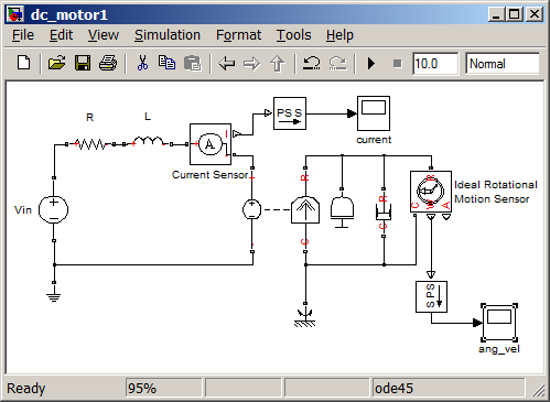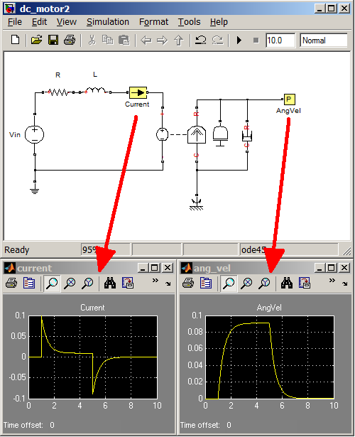It's very useful when your system starts to get very complicated, like an airplane or a car (yes, our customers use our tools to model whole aircrafts.) Those of you who have worked with physical systems can appreciate the fact that you can take measurements just by placing probes and sensors. Well, you can do that with a simulation model as well. To do that in Simscape, you place an appropriate sensor component, convert physical signals to Simulink signals, and measure.

It's pretty straight-forward once you understand the process, but with Tom's utility, sensing will now become second nature.

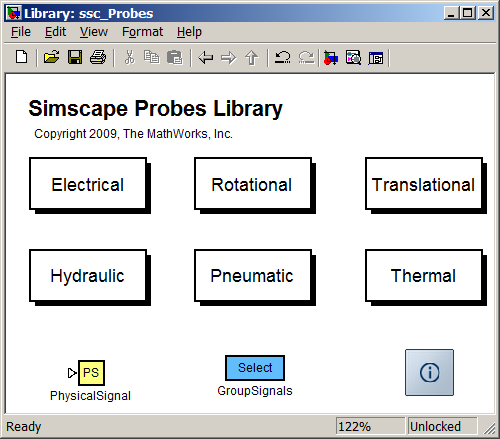
In addition to what you see above, he has created a slew of probes for various domains, a utility to group probe signals, and a help file.

Comments

Give this a try and tell us what you think, or leave a comment for Tom on the submission page.

Get the MATLAB code

Published with MATLAB® 7.9

Doug's picks this week are Simulink Support Packages for LEGO MINDSTORMS NXT [link], Beagleboard [link], Arduino Uno [link], and Arduino Mega [link] by the Classroom Resources Team.

This week, I'd like to highlight a new feature in the R2012a release of Simulink called Run on Target Hardware.

You may remember back in November 2010 Greg Wolff highlighted my Arduino Target submission that let you run a Simulink model on an Arduino Deumilanove by leveraging Simulink Coder and Embedded Coder to convert the model to C code.

So what's different about this new Run on Target Hardware capability? Well starting in R2012a you can now run your Simulink models on hardware even if you do not have Simulink Coder or Embedded Coder. That means that even those of you using the Student Version can take advantage of this capability! Run on Target Hardware currently supports the Uno and Mega varieties of the Arduino as well as the BeagleBoard-xM and LEGO MINDSTORMS NXT.

While there are File Exchange submissions for the supported hardware targets, you should install them directly from MATLAB by typing "targetinstaller" at the command prompt. This brings up a tool that automates the download and install process. Watch the video below to see it in action:

Introduction to Simulink Support for Target Hardware 1:57

Comments

We can't wait to see what kind of interesting projects you come up with by taking advantage of this capability. Please check it out and let us know what you think here.

San Diego

At the time of this posting, I will be in San Diego, California. I fully expect to be sitting on a beach or a sailboat getting a nice sunburn instead of shoveling snow off my driveway back in Massachusetts. Alright, who am I kidding, I'll be in a business meeting...

Out of curiosity to see where the planes would fly in order to transport us to Southern California, I turned to the File Exchange and discovered Simulink Dude's Flight Route Planning Simulator.

After downloading it there was a convenient run_me_now file that seemed, well, like I should run it!

My Own Flight Path

It appeared easy to change the example to use my flight termini. All I had to do was change the latitude and longitude vectors.

My flight itinerary is:

So I need to acquire the latitude and longitude of these cities, which could be done with an internet search. Instead, I'll do it completely within MATLAB using the Mapping Toolbox's new webmap functionality.

% Build the webmap.
h = webmap;

Now I need to zoom in on Logan, recording the airport coordinates. I did this interactively, and then extracted the center using wmcenter.

Repeating these steps for San Diego and Dallas yields latitude and longitude vectors of:

% Boston, San Diego, Dallas, Boston
latitude = [42.36532 32.73662 32.89819 42.36532].';
longitude = [-71.00800 -117.19137 -97.04380 -71.00800].';

% Add markers at the airports to check it
wmmarker(h,latitude,longitude);

Now I comment out the latitude and longitude vectors in the run_me_now script and then run it to use the ones I defined. This will pull up the Simulink Model and the Simulink 3D Animation virtual reality world viewer where we'll be able to see the flights:

How neat is that?

Plus, this also means I can now officially say: I've used the Aerospace Toolbox and Blockset :)

Comments

Give it a try and let us know what you think here or leave a comment for Simulink Dude.

Get the MATLAB code

Published with MATLAB® R2013b

This is probably one of the best documented submissions on the File Exchange. The Simulink models in this submission can be used to accurately simulate a commercial radio frequency (RF) chip (Analog Devices AD9361). The work was the result of collaboration between MathWorks and Analog Devices engineers, and the final result is a software model that matches the behavior of the physical device on the lab bench.

You can get a lot of details on the hardware and these software models here.

I will not go into any further technical details on this page, but I want to point out why I believe this was a useful and interesting project.

First, this is just plain cool! Seeing any software model predict (or match) hardware behavior at the level of detail that we find in these models is always interesting (having run simulations for 15+ years, I’m still amused when what I see in the lab matches what I predicted in simulation; it feels magical every time!)

Second, it helps understand and program the chip. An RF chip like the AD9361 (or most any chip for that matter) is a complex piece of hardware, and you can't see inside of it. This is an "agile" RF transceiver, which means it can be programmed to perform many different tasks for many different radio applications. Understanding the functioning of such a chip, and programming it correctly are rather difficult tasks in hardware, especially when the results of one's work can't be seen immediately (at least not without the use of expensive lab equipment such as spectrum analyzers). Having a software model that accurately mimics the hardware allows me to understand the behavior of the hardware such that I can program it better.

Third, debugging. If you have programmed anything but the simplest piece of hardware, you know that things rarely do what you want on the first try. Understanding apparent anomalies and hardware "misbehavior" is made infinitely easier when we can go to a simulation model and trace different signals to our heart"s content! With this Simulink model I can look at intermediate signals that I could never access on the physical chip. These intermediate signals often hold the key to understanding why the system’s outputs look the way they do.

Fourth (this should really be 3.5), studying the effects of an RF chip on digital baseband signals. These effects are generally something that we observe once we put everything together in the lab. Being able to simulate the digital baseband with the RF front-end will be quite useful in designing a robust communication system before we put any hardware together. Remember that as cool as physical prototypes are, they're typically quite expensive and time-consuming to build.

Finally (or fifth!), it builds trust in Simulink and SimRF. This one explains why we invested the time to do this. The fact that we could construct this model in a relatively short amount of time, and that it matches lab measurements, makes us confident that the simulation software tools are both capable and accurate.

I encourage you to take a look at the documentation and videos on this page to get more information on this package.

Comments

As always, your thoughts and comments here are greatly appreciated.

Get the MATLAB code

Published with MATLAB® R2014b

Contents

Organization is Everything!

Okay, maybe not everything. At some point you need to have substance in order to be useful. And documentation helps create the context in which to operate the tools. The Quad-Sim entry has all of these. The content of this entry is well organized in a way which helps detail what exactly is available within the content of the Quad-Sim tools.

In addition, the Simulink simulation models are well organized in terms of functional hierarchy. In other words, elements contained within the Simulink model are placed in well-named subsystems and libraries according to their functionality. There are clear partitions between inputs, controllers, plant dynamics, sensors, etc.

It sounds simple, but it makes all the difference. The organization of the content and the models alone made it very easy for me to understand, and start using the models.

I am definitely a proponent of Simulink as a platform for the development of dynamic systems and their control. Because I believe in Simulink as a design tool, it also means I spend a great deal of time and effort thinking about how to create and share models and supporting materials.

I have a self-imposed bias that makes it difficult for me to demonstrate or promote models that are messy, or otherwise difficult to understand. As such, I struggle to find File Exchange entries that involve Simulink, especially because Simulink is designed as a graphical tool, and therefore the form of the simulation model is at the forefront.

Documentation: The Asset Everyone Wants to Use, but No One Wants to Produce

If David and his colleagues somehow believe that the world of development and design will always be well thought-out and documented, they will soon be in for a shock.

Generally deadlines of overlapping projects loom, and we must produce functionality to meet specific needs now, and worry about documentation later (if at all).

As all of us know, being a user of a tool we want clear, well though-out documentation that not only has details of how to use a particular tool or feature, but examples of its use. Finally understanding the underlying nature of a particular feature helps us better use features appropriately. But as many of us are some sort of developer or designer, we also are aware of the effort required to produce such rigorous documentation.

The Quad-Sim not only has well written documentation on specifically how to use the included tools (e.g. Modeling GUI):

It also has detailed explanations of various experimental processes so they can be reproduced, and the tools can be understood relative to a specific design context (e.g. Motor Modeling Hardware).

Verification: Proof the Model Is Worth Building

The fact that David and his colleagues bothered to attempt and verify their system models really excited me. I know it sounds like maybe I should reconsider my priorities in life, but I couldn’t help showing some of my colleagues in my hall the Quad-Sim entry. Nor could I hide my excitement in seeing users spend the time to make sure their models are correct.

A model is an invaluable tool for design and analysis of complex systems. But what good is the use of that model for design if it is “wrong”?

Certainly “wrong” is a relative term. A model is always wrong, otherwise it’s not a model. I am specifically referring to the notion that a model must capture the important attributes of a system sufficiently with enough accuracy to be useful for the purposes of the design and analysis.

Maybe I should say: what good is using a model that is “too wrong”?

Code Generation for the Controller is an Excellent Next Step

It wasn’t clear to me that David and his colleagues used automated C-code generation from Simulink to implement the controller on the Arduino processor. Control systems like this are ideal candidates for our C-code generation technology from Simulink.

In my opinion, the Quad-Sim entry covers the more important aspects of the design process. It’s more important to get it right, without damaging people or equipment, than to implement quickly.

Seeing as that part of the process has been taken care of, it seems natural to me to automate the process of generating the control algorithm from the Simulink model to be implemented on the Arduino processor.

This enables two key design process attributes:

Both of these help save demand on software development resources, especially as designs become more complex, and design cycle iterations become shorter. We do offer an Arduino Hardware Support Package that enables you to include connections of the model to hardware peripherals such as analog-to-digital converters (ADC), and go all the way from the Simulink model to the executable running on the hardware with a single button click.

This is fine if you can represent the entire system software in Simulink. But in most cases, engineers want to integrate the control algorithm with some existing software framework. For this, you can leverage Embedded Coder to generate the C-code and then integrate the resulting code into your software project.

Okay That’s Enough Out of Greg Already!

I have lots of other comments and notions about this entry, but I’ll save that for other discussions. Let us know what you think.

Comments

If you would like to leave any comments regarding this post, please click here.

Get the MATLAB code

Published with MATLAB® R2014b

Contents

What is SimMechanics?

What is an S-function?

Are there other ways to do this?

How do they compare?

What do I like about this entry?

Do you need contact modeling in SimMechanics?

Get the MATLAB code

My pick this week is something that many of us could find useful and have likely thought about at some point during the standard workday: a simple design for the controller behind an automatically flushing toilet.

Techsource's Technical Team has put together a collection of simple Simulink models to showcase getting started with Simulink and an Arduino Board, a low cost embedded target.

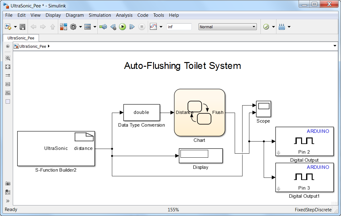
This particular one caught my attention for two reasons. First, the main model is called 'UltraSonic_Pee.slx'. If you want to grab someone's attention, well, a model name like this is a good way to do it. Second, this simple model is extensible so that I can include my own sensor input and simulate different flushing scenarios. Let's see how this is done.

Here's the original model:

For my Arduino board, I only have the LEDs and a simple DC motor. However, I have a Lego NXT that has an ultrasonic distance sensor and a DC motor that I can use. I don't know if the DC motor is actually powerful enough to pull down the handle on the urinal, but I'm going to try.

The first thing I am going to do is replace the two Arduino Blocks with a Lego Motor block from the Lego Support Package. Support packages are additional functionality you can freely download to allow MATLAB and Simulink to take advantage of your hardware.

One of the beautiful things about Simulink is the ability to have Variant Subsystems. These allow you to either have different fidelity models or to substitute in different components. My second step is going to be to make the Signal Builder block into a variant subsystem so I can have my Lego distance sensor as an input instead. This is really important for the modeling aspect. I'm fortunate enough right now to have access to the hardware. But if I did not, I could still develop and test my algorithms by simulating the hardware with other signals that I could build or historical data from other tests.

Next I'm going to simulate this in External Mode. This means that the model will be running in Simulink but be grabbing data from the sensors and controlling the motor. By running in External Mode we can use the full power of the MATLAB and Simulink platforms to analyze the results of the model and see it running in semi-real-time. By doing this, I discovered that I needed a couple of gains on the signals to control how close one needs to get to trip the sensor.

Once the model has been tested, we can then embed the controller onto the Lego. One button click in Simulink generates the equivalent C-code, compiles it, and moves it onto the Lego.

Now we're ready to put this to the test!

The looks we got from fellow restroom patrons and the cleaning staff were pretty priceless.

Next I got my friend Adam, who is relocating from Massachusetts to California shortly, to test it out. The control algorithm that Techsource used is to have a preflush and a postflush - not the most environmentally friendly of algorithms but we waste no water in simulation. Since this is no longer simulation, I figured Adam should enjoy this luxury while still being on the east coast.

Unfortunately, the Lego motor was not strong enough to pull the handle down and instead lifted the whole robot up. But hey, not too shabby for an hour's worth of work.

Comments

Give it a try and let us know what you think here or leave a comment for the Techsource Technical Team.

Get the MATLAB code

Published with MATLAB® R2015a

Pick

My pick this week is Developing Simulink Device Driver Blocks: Step-by-Step Guide and Examples .

One of the many capabilities of Simulink is the ability to generate code for an embedded application. However, when hardware is involved, the complexity goes up exponentially. As with any embedded system, the core algorithm must interface with hardware components to be effective. These can range from simple I/O, to complex sensors such as a GPS. In addition, there are myriad communication channels that can be used such as serial, A2D/D2A, and other communication protocols (i.e. I2C). In all of these cases, there are some low-level hardware routines that provide a bridge between the hardware and the core algorithm - device drivers.

That being said, the issue then becomes how do you call these low-level routines? One way would be to write all of the code by hand. This is not very efficient and not recommended. Another would be to write the base code for the application by-hand, including the interface to the hardware, and calling the algorithmic code produced via Simulink. In reality, this is an approach adobted by many users, particularly where it is a highly complex system with many aspects, with a limited number being generated from Simulink. However, for our case, we want to be able to generate code from our Simulink model and run it directly on our hardware, especially if we are using the Run on Target Hardware feature in Simulink rather than using one of the Coder products. To do this, we need a block in Simulink that will translate into a call to the appropriate device driver.

That is where this post comes into play. This post walks you through the steps needed to create these device driver blocks. In particular, the post provides information on the various approaches that can be used such as S-Function blocks and MATLAB Function blocks, and the pros/cons of each approach. The post provides examples for creating blocks for an Arduino board, but the approach is applicable to any board. This is supported by the number of additional posts that were inspired by this post for a wide range of boards and applications.

Once a device driver block is created, the user can place it in a Simulink library for reuse. In this way, various device driver blocks can be packaged and shared for use in different applications. Many of the Target Support Packages leverage this capability.

Comments

If you need to interface with hardware, this post can provide the necessary guidance to allow you to create a set of hardware specific blocks. Give it a try and let us know what you think here or leave a comment for Giampiero.

Get the MATLAB code

Published with MATLAB® R2016a

Data Acquisition Hardware

Have you ever wanted to bring data directly from hardware into MATLAB or control something via a data acquisition board?

Working with data acquisition hardware was my very first project in MATLAB back in the winter of 2008. I had a miniature load frame, transparent to x-rays, for applying a load to a concrete cylinder. There were three sensor inputs: two displacements, and force, and one output: a voltage to a piezoelectric actuator that applied a force. Here's a figure from my thesis:

I built a user interface in GUIDE to allow me to apply the load while recording and plotting the signals. To complicate matters, the session based interface for the Data Acquisition Toolbox didn't exist yet, so I was also doing everything with timers on my own.

I can only imagine how much easier it would've been with this app. I no longer have access to the load frame, so instead here's an example getting data from an ADALM1000, a low cost data acquisition device.

Let's control it with the app. First, I'll just get connected and pull some data from the attached RC circuit. Note I previously had to install the hardware support package for this board.

Seems to work, great!

Now I want to output some data to it. There are two channels, the first will be a sine wave and the second a cosine wave. The board can take 0-5V so add 1 to the waves keep them positive.

t = linspace(0,8*pi,100000)';
x = [sin(t) cos(t)]+1; %

In order to get them into the output, we simply pick the variable:

And then run the session:

From here, the data can be exported or equivalent code can be generated from the file menu to automate this acquisition session.

My only point of feedback is that error messages are not all exposed via dialogs. For example, the first time I selected x with the range -1:1, it errored at the command line with a useful message that I didn't see because the app was maximized.

Going back to my use case in college, I was trying to control load, with displacement so that the loading rate would be roughly linear. To do this, I ran a bunch of experiments and fit an equation to the load v. displacement curve for many cylinders. At the time, I knew nothing about Simulink or how it could help me. If challenged with the same task today, I would likely use the data acquisition blocks in Simulink R2016b to control the actuator. This would allow me to then use the PID block and its tuning capabilities to accomplish what I was doing much more quickly.

For nostalgia's sake, I put together a quick a model of the system.

Comments

Do you work with data acquisition hardware? Give it a try and let us know what you think here or leave a comment for Isaac.

Get the MATLAB code

Published with MATLAB® R2016b

Contents

What is SimMechanics?

What is an S-function?

Are there other ways to do this?

How do they compare?

What do I like about this entry?

Do you need contact modeling in SimMechanics?

Get the MATLAB code